| Ch 8. Incompressible and Viscous Flow | Multimedia Engineering Fluids | ||||||
|
Flow between Parallel Plates |
Couette Flow |
Viscous Flow in Pipe |
|||||
| Viscous Flow in Pipe | Case Intro | Theory | Case Solution | Example |
| Chapter |
| 1. Basics |
| 2. Fluid Statics |
| 3. Kinematics |
| 4. Laws (Integral) |
| 5. Laws (Diff.) |
| 6. Modeling/Similitude |
| 7. Inviscid |
| 8. Viscous |
| 9. External Flow |
| 10. Open-Channel |
| Appendix |
| Basic Math |
| Units |
| Basic Fluid Eqs |
| Water/Air Tables |
| Sections |
| eBooks |
| Dynamics |
| Fluids |
| Math |
| Mechanics |
| Statics |
| Thermodynamics |
| ©Kurt Gramoll |
|
|
|||||||||||||||||||||||||||||||
|
This section begins with a brief review on laminar and turbulent flows followed by an introduction of fully developed flow. The Hagan-Poiseuille and Darcy-Weisbach equations are then presented for circular pipe flow. In this section, the pipe is assumed to be fully occupied by the fluid and the pressure in the fluid is greater than zero gauge. Flows in partially filled pipes are covered in the discussion of open channel flow. At the end of this section, flow in non-circular conduits is discussed. |
|||||||||||||||||||||||||||||||
| Entrance and Fully Developed Regions |
|||||||||||||||||||||||||||||||
|
|
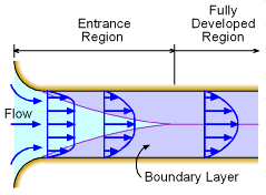
Recall that Reynolds number (Re = ρVD/μ) can be used to classify if a flow is laminar or turbulent. The type of flow not only depends on its velocity (V), but also its density (ρ), viscosity (μ) and length scale (diameter D). For pipe flow, the flow is laminar when Re < 2,100, and it is turbulent when Re > 4,000. The flow is referred to as transition flow when Reynolds number is in between 2,100 and 4,000. When a fluid enters a pipe, viscous effects due to the pipe wall will develop. The region where viscous effects are important is referred to as the boundary layer. The velocity profile, as shown in the figure, will also vary due to the growth of this boundary layer. When the velocity profile reaches a constant (i.e., velocity profile no longer changes along the pipe), the flow is said to be fully developed. The length required for the flow to reach fully developed conditions is called the entrance length (Le), and it can be determined from the following empirical relations: For laminar flow: Le/D = 0.06Re For turbulent flow: Le/D = 4.4(Re)1/6 |
||||||||||||||||||||||||||||||
| Hagan-Poiseuille Flow |
|||||||||||||||||||||||||||||||
|
|
Fully developed laminar pipe flow is generally known as Hagan-Poiseuille flow. The velocity profile of a fully developed laminar horizontal circular pipe flow can be derived from the Navier-Stokes equations and is given by The derivation process is similar to that of obtaining the velocity distributions for
flow between parallel plates, hence the derivation details
are omitted here for brevity. The assumptions used in the derivation are as follows: The obtained velocity profile is parabolic, and it closely resembles the velocity profile obtained for flow between parallel plates. The volumetric flow rate (Q) can then be determined by integrating the velocity profile over the cross-sectional area to yield: |
||||||||||||||||||||||||||||||
| Darcy-Weisbach Equation |
|||||||||||||||||||||||||||||||
|
From another discussion, it is known that Bernoulli's equation can be applied along a streamline to analyze steady, incompressible and inviscid flow. Most flows in real practice, however, are viscous, and hence losses due to viscous dissipation (friction) are unavoidable. To analyze flow in a viscous pipe, Bernoulli's equation can be modified and applied to two sections of the pipe flow: where p is the static pressure, V is the average velocity, z is the elevation, and hL accounts for the head loss due to friction between section (1) and (2). |
||||||||||||||||||||||||||||||
|
Table: Typical Values of Surface Roughness
|
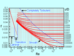
Based on dimensional analysis, the head loss over the length of the pipe is given by where f is an empirical friction factor. The above expression is also called the Darcy-Weisbach equation. The friction factor is a function of the Reynolds number (Re) and relative roughness of the pipe (ε/D) as shown in the Moody chart to the left. Typical values of the surface roughness of pipe (ε) are summarized in the table. The Moody Chart actually has three main regions or sections. The first region is for laminar flow for when Re is approximately less than 2100. Then the friction factor is a a direct function of the Re, or For laminar flow: f = 64/Re The region between laminar and completely turbulent. This is when the chart is required. First determine the relative roughness number, ε/D, and then determine Re. Using these two numbers and the Moody Chart, estimate the friction factor, f. In general, the friction factor is a function of Re and ε/D for turbulent flow. However, when Re is very high (completely turbulent flow), the friction factor becomes independent of Re, and it depends on the relative roughness only. This is the third region and as an alternative to determining the friction factor for turbulent flow from the Moody chart, it can be calculated using the correlation provided by Colebrook**, For turbulent flow: Note that iteration is needed to obtain f since the above equation is not expressed explicitly in f. [**Reference: Colebrook, C. F., "Turbulent Flow in Pipes with Particular Reference to the Transition between the Smooth and Rough Pipe Laws," Journal of the Institute of Civil Engineering London, Vol. 11, pp. 133-156, 1939.] |
||||||||||||||||||||||||||||||
|
|
Flow in Non-Circular Conduits |
||||||||||||||||||||||||||||||
To analyze flow in conduits with non-circular shapes, the hydraulic diameter (Dh) can be used in place of the diameter. It is defined as Dh = 4A/P where A is the cross-sectional area, and P is the wetted perimeter. |
|||||||||||||||||||||||||||||||


